Introduction
Path tracking and obstacle avoidance are two very important behaviours that must be considered in the process of developing Autonomous Ground Vehicles, AGV.There are many well known path tracking algorithms, like follow-the-carrot and pure-pursuit, as well as the more recently developed vector-pursuit tracking method.
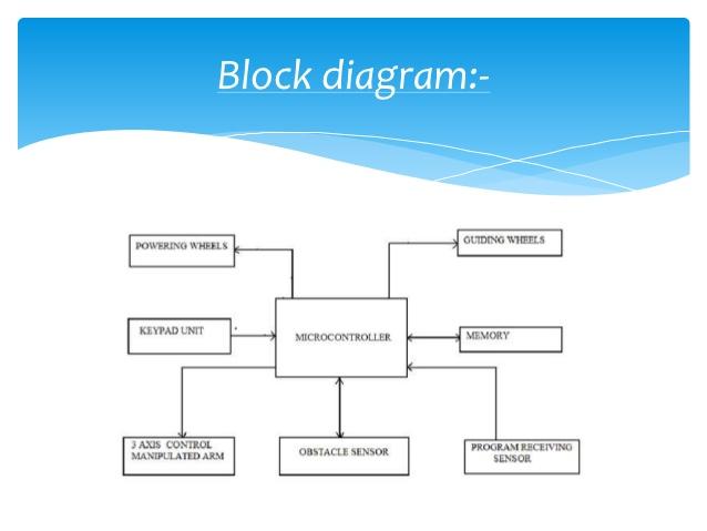
The following Block diagram will give you the gist of this tutorial.
Dead reckoning
Dead reckoning is a method used for determining the current position of a vehicle, by advancing some previous position through known course and velocity information over a given time period. Most of the robotic ground vehicles today rely on dead reckoning as the framework of their navigational systems. One simple way to implement dead reckoning is called odometry. Odometry is a method to provide information about vehicle displacement based on the rotation of its motors or wheels. The rotation is measured by wheel or shaft encoders. These encoders counts the number of rotations of the wheel axles, providing data that combined with the forward kinematics equations can be translated to information regarding the change in position and heading of the vehicle. Figure below shows a picture of the normal configuration and placement of encoders and motors on a differential drive ground robot vehicle.
Differential drive kinematics
The theory behind differential drive kinematics is pretty straightforward. Every wheeled mobile robot in a state of motion must always rotate about a point that lies somewhere on the common axis of the two wheels. This point is often called the instantaneous centre of curvature (ICC), or the instantaneous centre of rotation (ICR). A differential drive robot changes the position of the ICC simply by varying the velocities of the two wheels. Two separate drive motors, one for each wheel, provide independent velocity control to the left and right wheels. It is this property that makes it possible for the robot to choose different trajectories and paths. A sketch describing the kinematics of a differential drive mobile robot can be seen in figure below.
VARIOUS ALGORITHMS
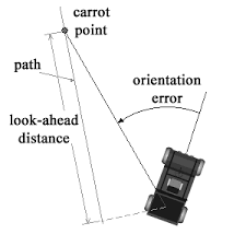
1.Follow-the-carrot
This algorithm is based on a very simple idea. Obtain a goal-point, then aim the vehicle towards that point. Figure below describes the basics behind this method.
2.Pure Pursuit
The concept of the pure pursuit approach is to calculate the curvature that will take the vehicle from its current position to a goal position. The goal point is determined in the same manner as for the follow-the-carrot algorithm. A circle is then defined in such a way that it passes through both the goal point and the current vehicle position. Finally a control algorithm chooses a steering angle in relation to this circle. Infact, the robot vehicle changes its curvature by repeatedly fitting circular arcs of this kind, always pushing the goal point forward.
I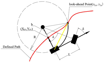
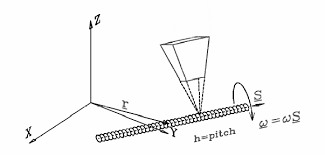
3.Vector Pursuit
Vector pursuit is a new path tracking method that uses the theory of screws first introduced by Sir Robert S. Ball in 1900. Screw theory can be used to represent the motion of any rigid body in relation to a given coordinate system, thus making it useful in path tracking applications. Any instantaneous motion can be described as a rotation about a line in space with and associated pitch.
The look-ahead distance
Common to all these methods is that they use a look-ahead point, which is a point on the path a certain distance L away from the orthogonal projection of the vehicle’s position on the path. Changing the look-ahead distance can have a significant effect on the performance of the algorithm. There are two problems that need to be considered:
-
Regaining a path
-
Maintaining the path
The first problem occurs when the vehicle is way off the path, thus having large positional and orientation errors, and is trying to return to this path. A larger value causes the vehicle to converge more smoothly and with less oscillations. On the other side, once back on the path a large value will lead to worse tracking, especially in the case of paths containing very sharp curves.
Factors to be considered while choosing the look-ahead distance
-
Vehicle Speed
-
Is the path obstacle free
Obstacle Avoidance
The obstacle avoidance unit is a simple local implementation based entirely on proximity sensors. We can implement some kind of global obstacle avoidance algorithm, like the Potential Field method or the Vector Field Histogram method or local ones. The global methods are better but they require more accurate ultrasonic sensors.
Give below is an example of a local method of obstacle avoidance :
During the tracking phase the obstacle avoidance unit is responsible for repeatedly checking the four proximity sensors in the front. If any obstacles are detected the robot stops, rotates 90 degrees in some direction, and thereafter follows the edge of the obstacle until it points towards the current goal point again and no obstacle are in front of the robot. Thus the obstacle avoidance unit consists of three phases:
- Stop
- Rotate
- Follow edge
A stop and rotate phase may seem unnecessary, but I saw no other possibility considering the bad accuracy of the proximity sensors. These sensors can only detect obstacles at a maximum distance of approximately three centimetres, so without these phases the robot would bump into the obstacle instead of avoiding it.