Introduction
Shape detection is an important part of Image Processing referring to modules that deal with identifying and detecting shapes of parts of image which differ in brightness,color or texture. There are several reasons we need to study shape detection most important being identifying shapes in images for object recognition or feature detection/extraction.
Shape detection is usually done after blob detection i.e. once the blob details are obtained and it can be processed to find shape of the blob for further classification of blobs. There are various advanced means of shape detection and research is still going on to find even better algorithms for the same. However, OpenCV already has used one of the most widely used algorithms called Hough Transform for some shapes like lines, circles, ellipse and squares.
Algorithm - Hough Transform
The purpose of the technique is to find imperfect instances of objects within a certain class of shapes by a voting procedure. This voting procedure is carried out in a parameter space, from which object candidates are obtained as local maxima in a so-called accumulator space that is explicitly constructed by the algorithm for computing the Hough transform.
In automated analysis of digital images, a sub-problem often arises of detecting simple shapes, such as straight lines, circles or ellipses. In many cases an edge detector can be used as a pre-processing stage to obtain image points or image pixels that are on the desired curve in the image space. Due to imperfections in either the image data or the edge detector, however, there may be missing points or pixels on the desired curves as well as spatial deviations between the ideal line/circle/ellipse and the noisy edge points as they are obtained from the edge detector. For these reasons, it is often non-trivial to group the extracted edge features to an appropriate set of lines, circles or ellipses. The purpose of the Hough transform is to address this problem by making it possible to perform groupings of edge points into object candidates by performing an explicit voting procedure over a set of parameterized image objects.
Hough Lines
The simplest case of Hough transform is the linear transform for detecting straight lines. In the image space, the straight line can be described as y = mx + b and can be graphically plotted for each pair of image points (x, y). In the Hough transform, a main idea is to consider the characteristics of the straight line not as image points (x1, y1), (x2, y2), etc., but instead, in terms of its parameters, i.e., the slope parameter m and the intercept parameter b. Based on that fact, the straight line y = mx + b can be represented as a point (b, m) in the parameter space. However, one faces the problem that vertical lines give rise to unbounded values of the parameters m and b. For computational reasons, it is therefore better to use a different pair of parameters, denoted and (theta), for the lines in the Hough transform. These are the Polar Coordinates.
The parameter represents the distance between the line and the origin, while is the angle of the vector from the origin to this closest point. Using this parameterization, the equation of the line can be written as
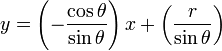
which can be rearranged to .
It is therefore possible to associate with each line of the image a pair (r,θ) which is unique if  and
and  , or if
  and
and  . The (r,θ) plane is sometimes referred to as Hough space for the set of straight lines in two dimensions.
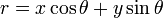
For an arbitrary point on the image plane with coordinates, e.g., (x0, y0), the lines that go through it are the pairs (r,θ) with,

where (the distance between the line and the origin) is determined by θ.
This corresponds to a sinusoidal curve in the (r,θ) plane, which is unique to that point. If the curves corresponding to two points are superimposed, the location (in the Hough space) where they cross corresponds to a line (in the original image space) that passes through both points. More generally, a set of points that form a straight line will produce sinusoids which cross at the parameters for that line. Thus, the problem of detecting collinear points can be converted to the problem of finding concurrent curves.
Implementation
The Hough transform algorithm uses an array, called an accumulator, to detect the existence of a line y = mx + b. The dimension of the accumulator is equal to the number of unknown parameters of the Hough transform problem. For example, the linear Hough transform problem has two unknown parameters: the pair (m,b) or the pair (r,θ). The two dimensions of the accumulator array would correspond to quantized values for (r,θ). For each pixel and its neighborhood, the Hough transform algorithm determines if there is enough evidence of an edge at that pixel. If so, it will calculate the parameters of that line, and then look for the accumulator’s bin that the parameters fall into, and increase the value of that bin. By finding the bins with the highest values, typically by looking for local maxima in the accumulator space, the most likely lines can be extracted, and their (approximate) geometric definitions read off. (Shapiro and Stockman, 304) The simplest way of finding these peaks is by applying some form of threshold, but different techniques may yield better results in different circumstances - determining which lines are found as well as how many.
Since the lines returned do not contain any length information, it is often next necessary to find which parts of the image match up with which lines. Moreover, due to imperfection errors in the edge detection step, there will usually be errors in the accumulator space, which may make it non-trivial to find the appropriate peaks, and thus the appropriate lines.
The result of the Hough transform is stored in a matrix that often is called an accumulator. One dimension of this matrix are the angles θ and the other dimension are the distances r, and each element has a value telling how many points/pixels are positioned on the line with parameters (r,θ). So the element with the highest value tells what line that is most represented in the input image.
Consider three data points, shown here as black dots.
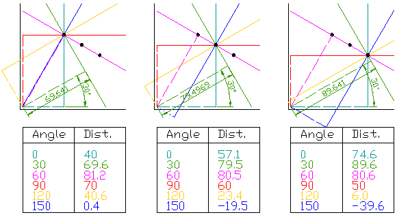
- For each data point, a number of lines are plotted going through it, all at different angles. These are shown here as solid lines.
- For each solid line a line is plotted which is perpendicular to it and which intersects the origin. These are shown as dashed lines.
- The length (i.e. perpendicular distance to the origin) and angle of each dashed line is measured. In the diagram above, the results are shown in tables.
- This is repeated for each data point.
- A graph of the line lengths for each angle, known as a Hough space graph, is then created.
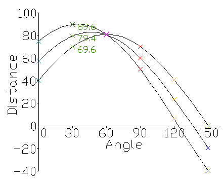
The point where the curves intersect gives a distance and angle. This distance and angle indicate the line which intersects the points being tested. In the graph shown the lines intersect at the pink point; this corresponds to the solid pink line in the diagrams above, which passes through all three points.
A similar approach using suitable parameters can be done easily for shapes like circles, ellipse and squares.
There are predefined Hough functions for lines, circle and ellipse using cvHoughlines2, cvHoughcircles etc about which you can get from the book Learning OpenCV - Computer Vision with the OpenCV library - Gary Bradski and Adrian Kaehler. The book is available for free online.