Kalman Filter is an algorithm that uses series of measurement observed over time containing noises and other inaccuracies to predict best estimate of unknown variables that tend to be more accurate than a single measurement. There are many modifications in kalman filter resulting in new algorithm such as extended kalman filter (EKF) and unscented kalman filter. These models work on non linear systems. Following tutorial is on KF which works on linear system .To understand kalman filter you should be thorough with basics of normal distribution and little bit of linear algebra.
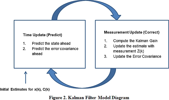
In kalman filter we assume that all measurements and noises are probabilistic and have some mean and co variance. Kalman filter can be divided into two basic operations : 1.Prediction 2.Update An initial estimate is given then after that it continuously goes in loop between the two processes .
Lets start understanding it with a simple example.
To understand what it does, take a look at the following data - if you were given the data in blue, it may be reasonable to predict that the green dot should follow, by simply extrapolating the linear trend from the few previous samples. However, how confident would you be predicting the dark red point on the right using that method? how confident would you about predicting the green point, if you were given the red series instead of the blue? 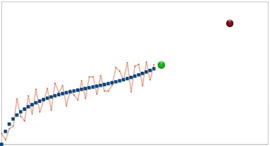 Now, let’s try and use the above to model our prediction.
First we need to know the state of our system. State of system is the vector of parameters that we need to know to completely describe the system.For example if our system consists of car moving in one dimension then state of the system would be position and velocity of the car. In our case we will take y coordinate and slope as our state. It is generally denoted by x. The next thing we need is model for our system .It describes how our system behaves.In our case it is y(t)=y(t−1)+m(t−1) and m(t)=m(t−1) where t represents time. Expressing in matrix form
$ x_t = \begin{bmatrix}y(t)\\ m(t)\end{bmatrix} = \begin{bmatrix} 1 & 1 \\ 0 & 1 \end{bmatrix}.\begin{bmatrix} y(t-1) \\ m(t-1) \end{bmatrix} = Fx_{t-1}$
But our system would not be perfect so there must be noise known as state noise $v_t$ . It is assumed to be white noise(normally distributed with mean zero and some covariance). So our equation becomes
$x_t = \begin{bmatrix} y(t) \\ m(t) \end{bmatrix} = \begin{bmatrix} 1 &1 \\ 0 & 1 \end{bmatrix}.\begin{bmatrix} y(t-1) \\ m(t-1) \end{bmatrix} = Fx_{t-1} + v_t$
One final equation that we are missing with is measurement update equation. $measurement = \begin{bmatrix} 1 & 0 \end{bmatrix}.\begin{bmatrix} y(t) \\ m(t) \end{bmatrix}$
Again there will be some noise in the measurements we denote it with $w_t$It is also a white noise. $z_t = \begin{bmatrix} 1 & 0 \end{bmatrix}.\begin{bmatrix} y(t) \\ m(t) \end{bmatrix} + w_t$ In kalman filter everything is represented by normal distribution. Applying mean value of operator on both the side of equations we get
${x_t} = \begin{bmatrix} y(t) \\ m(t) \end{bmatrix} = \begin{bmatrix} 1 &1 \\ 0 & 1 \end{bmatrix}.\begin{bmatrix} y(t-1) \\ m(t-1) \end{bmatrix} = Fx_{t-1} $———- (1) (mean of $v_t$ is zero)
$z_t = \begin{bmatrix} 1 & 0 \end{bmatrix}.\begin{bmatrix} y(t) \\ m(t) \end{bmatrix} = H.x_t $ ————- (2) (mean of $w_t$ is zero) F is known as state transition model .It is designed according to your system. H is observation model. So we predict our state after time t with equation 1 and the expected measurement is given buy equation 2 .But our expected measurement and true measurement will not match because if that would happen we would not need a kalman filter. Let us assume we measured some value represented by matrix ${a_t}$. Let y represent the error between them, then y = ${a_t} - z_t $
To incorporate this into our model, we add the innovation to our state equation, multiplied by a matrix factor that tells us how much the state should change based on this difference between the expected and actual measurements. ${x_t} = Fx_{t-1} + Wy $
W is called kalman gain. Now calculating this is the point where things become little bit confusing. Now suppose we have a high process noise , it means there is a strong tendency for the system to change rapidly. Therefore innovation should be taken seriously (means there can be difference between our predicted and measured value as system is changing rapidly). This implies W should be large and directly proportional to process noise. But if we have a high measurement noise it is not necessary that our system might have changed ,it can also be wrong data as we have high measurement noise. So W can be said to be inversely proportional to measurement noise.
W ~ (process noise)/(measurement noise)
Now we have to calculate the noises. The best way to represent the noise is variance. For calculating process noise we will take co-variance of $x_t$. $P_t$ = Cov($x_t$) = Cov($Fx_{t-1}$) =$F$.Cov($x_{t-1}$).$F^T$ =$F.P_{t-1}.F^T$ However , this assumes our process model is perfect and there’s nothing we couldn’t predict. But normally there are many unknowns that might be influencing our state (maybe there’s wind, friction etc.). We incorporate this as a covariance matrix Q of process noise $v_t$ and prediction variance becomes: $P_t = F.P_{t-1}.F^T + Q$
Similarly for measurement noise $S_t = Cov(z_{t})$ $S_t = H.P_t.H^T + R$ So we get $ W = P_{t}.H^T.S_t^{-1}$
One more way to understand kalman gain is that suppose we have highly faulty instruments and we can’t rely on there readings so in that case our prediction is supposed to be more accurate .Rewriting our kalman gain equation ${x_t} = Fx_{t-1} + W ({a_t} - z_t {x_t}) = Fx_{t-1} + W ({a_t} - H.F.x_{t-1}) $
So our W should be such that $a_t$ has less weight-age and $x_{t-1}$ has more which implies that W should be small. Similarly we can show that if our measurement noise is less W should be large. Finally we have to update the error co-variance
$P_t = (I - K.H).P_t$
Summarising 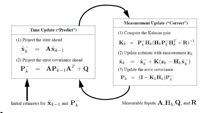
In the above image A is the same matrix as F that is given in the derivation above.
The derivation that was given above is not completely mathematical but it is easy to understand and know what is happening in kalman filter.
For proper mathematical derivation links are given below which you can refer.